Two Stream Instability
Introduction to plasma two stream instsability with code
What is two stream instability ?
Consider a system comprising two types of fluid, which can be either cold or hot electron beams, moving through a periodic domain with a length of L.
We’ll first derived the linear behavior of the instability then verified the theory by applying Particle-in-Cell simulation which follow closly with 1985 Berkely Plasma Physics via Computer Simulation for more comprehensive derivation.
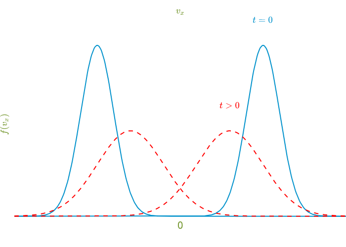
Visulization
First, let’s examine the outcomes of the simulation.
Theory
Governing Equations
The system is described using:
- Electrostatic wave ↔ Electron motion
- Vlasov (equation of motion) + Continuity Equation + Poisson’s equation
The fundamental equations are:
\[f(x, v, t) = v\] \[\frac{\partial v}{\partial t} + v \frac{\partial v}{\partial x} = - \frac{e}{m_e} E\] \[\frac{\partial n}{\partial t} + \frac{\partial (nv)}{\partial x} = 0\] \[\frac{\partial E}{\partial x} = - \frac{e}{\varepsilon_0} (n - n_0)\]Where:
-
vis the velocity of the electron fluid, -
nis the density of the electron fluid, -
n_0is the density of the ion background.
Case 1
Consider small perturbations of density, velocity, and field in a stationary background.
First, we consider the case where E0 = 0 and v0 = 0, combine the govern equations and keeping only linear terms we have:
Then, we assume the traveling wave solution which is proportional to \(e^{i(kx - \omega t)}\). We have:
\[i \omega v_1 = -\frac{e}{m_e} E_1\] \[-i \omega n_1 + i n_0 k v_1 = 0\] \[i k E_1 = -\frac{e}{\varepsilon_0} n_1\]We have
\[\left( 1 - \frac{n_0 e^2}{\varepsilon_0 m \omega^2} \right) E_1 = 0\] \[\left( 1 - \frac{\omega_p^2}{\omega^2} \right) E_1 = 0\]For a nontrivial solution:
\[\omega = \pm \omega_p\]This is consistent with our physical picture, where the electrostatic wave frequency equals the plasma frequency.
Case 2
In another situation where the electron fluid has a velocity (v0 ≠ 0), the governing equations become:
Assuming a plane wave solution, we have:
\[\left[ 1 - \frac{\left( \omega_p^2 / \omega^2 \right) - k v_0}{2} \right] E_1 = 0\] \[\omega = \omega_D \pm \omega_p\]Where \(\omega_D\) represents the Doppler frequency, indicating that the plasma oscillation frequency is shifted by the Doppler effect.
Combine Case 1 and 2
This scenario consists of two electron fluid species: one relatively stationary to the ion background, and another with velocity \(v_0\). For plasma neutrality, we require:
\[n_0 = n_{01} + n_{02}\]The Vlasov and continuity equations are the same as in the previous cases (3) and (8), but Poisson’s equation is coupled together by the two fluids:
\[\frac{\partial E_1}{\partial x} = -\frac{e}{\varepsilon_0} (n_{11} + n_{12})\]By substituting \(n_{11}\) and \(n_{12}\) with the Vlasov and continuity equations, we obtain:
\[\left[ \frac{n_{01} e^2}{m \varepsilon_0 \omega^2} + \frac{n_{02} e^2}{m \varepsilon_0 (\omega - \omega_D)^2} - 1 \right] E_1 = 0\]Finally, the dispersion relation can be expressed as:
\[F(\omega) \equiv \frac{\omega_{p1}^2}{\omega^2} + \frac{\omega_{p2}^2}{(\omega - \omega_D)^2} = 1\]Where \(\omega_{p1}\) and \(\omega_{p2}\) are the plasma frequencies of the two species.
For \(\omega_D >> 0\) (right figure)
\[F(\omega) = \frac{\omega_{p1}^2}{\omega^2} + \frac{(\omega - \omega_{p2}^2)^2}{(\omega - \omega_D)^2} = 1\]
The solution is \(\omega \approx \pm \omega_{p1} \quad \omega \approx \omega_D \pm \omega_{p2}\)
We look for the minimum of \(F\left( \omega \right)\) which happens at
\[\omega = \omega_m = \omega_D \left[1 + \left(\frac{\omega_{p2}}{\omega_{p1}}\right)^{2/3}\right] \equiv \omega_D \left(1 + \alpha^{2/3}\right)\]where \(\alpha \equiv \frac{\omega_{p2}}{\omega_{p1}}\)
For \(\omega_D \approx 0\)
Then the minimum of function \(F\left( \omega \right)\) is
\[F_m = F(\omega_m) = \frac{\omega_{p1}^2}{\omega_D^2} \left(1 + \alpha^{2/3}\right)^3\]
Let’s assume that \(n_{02} \ll n_{01}\), \(\omega_{p2} \ll \omega_{p1} \quad \text{and} \quad \alpha \ll 1.\)
\[F_m \approx \frac{\omega_{p1}^2}{\omega_D^2} \left(1 + 3\alpha^{2/3}\right)\]So then if
\[\frac{\omega_{p1}^2}{\omega_D^2} < \left(1 + 3\alpha^{2/3}\right)\text{,} \quad F_m < 1 \quad \Rightarrow \quad 4 \text{ real roots.}\] \[\frac{\omega_{p1}^2}{\omega_D^2} > \left(1 + 3\alpha^{2/3}\right)\text{,} \quad F_m > 1 \quad \Rightarrow \quad 2 \text{ real + 2 complex roots.}\] \[\Rightarrow \quad \omega = \omega_{re} \pm i\omega_{im}\]It will have the solution of \(E \propto e^{i(kx - \omega_{re} t)} e^{\omega_{im} t}\) which grows in time.
The instability happened roughly at
\[v_f \approx v_0\]When phase velocity is close to fluid velocity, the coupling effect between electrons and wave becomes very strong. With \(v_0\) slightly larger than phase velocity, the energy of the electron is easily transferred to the wave, which results in the positive feedback growth of the electrostatic wave.
Two stream instability
Instability occurs when \(F(\omega_m) > 1\) when \(\omega_{p1} = \omega_{p2} = \omega_p\) it gives us
\[\frac{\omega_p^2}{\omega_D^2} > \frac{1}{8}\]And defining \(\beta \equiv \frac{\omega_D}{\omega_p}\) we have the following instability condition:
\[\beta < \sqrt{8}\]Which is verified by directly solving the dispersion relation.
\[\frac{\omega_p^2}{\omega^2} + \frac{\omega_p^2}{\left( \omega - \omega_D \right)^2} = 1\]
Simulation
Temporal grid
\[\frac{d\mathbf{r}_i}{dt} = \mathbf{v}_i, \quad \frac{d\mathbf{v}_i}{dt} = - \frac{e}{m_e} \mathbf{E}(\mathbf{r}_i)\] \[\mathbf{E}(\mathbf{x}) = \sum_i \frac{1}{4\pi\epsilon_0} \frac{e}{r_i^2}\]In this scheme we only need two steps to implement this simulation: first find the electric field and then integrate the equation of motion. Combine these two procedures we have formed the temporal grid. However, this process is time-consuming (e.g., for N particles it has the computation complexity of \(\approx 2N + N(N - 1)/2\)).
| Method | complexity |
|---|---|
| Temporal Grid | \(\approx N^2/2 + N\) |
| PIC | \(4N\) |
Temporal grid and Spatial grid
A better way is to simplify the process of calculating the electric field since plasma provides shielding that only the particles within a few nearby Debye cubes are significant. We don’t need all the information of particles to calculate the electric field. Instead, we divide the space into a spatial grid that stores the information regarding density (\(\rho\)), potential (\(\phi\)), and field (\(E\)).
In this scenario, we are equivalent to solving the following four equations:
\[\frac{d\mathbf{r}_i}{dt} = \mathbf{v}_i, \quad \frac{d\mathbf{v}_i}{dt} = - \frac{e}{m_e} \mathbf{E}(\mathbf{r}_i)\] \[\mathbf{E}(\mathbf{x}) = -\frac{d\phi(\mathbf{x})}{dx}, \quad \frac{d^2\phi(\mathbf{x})}{dx^2} = \frac{e}{\epsilon_0} (n_0 - n(\mathbf{x}))\]Temporal grid, Spatial grid and Finite difference
Changing the first and second-order ODE into finite difference form:
\[\frac{d\mathbf{r}_i}{dt} = \mathbf{v}_i\] \[\frac{d\mathbf{v}_i}{dt} = - \frac{e}{m_e} \mathbf{E}(\mathbf{r}_i)\] \[\mathbf{E}(\mathbf{x}) = -\frac{d\phi(\mathbf{x})}{dx} = \frac{\phi_{j-1} - \phi_{j+1}}{2\Delta x}, \quad \frac{d^2\phi(\mathbf{x})}{dx^2} = \frac{\phi_{j-1} - 2\phi_j + \phi_{j+1}}{(\Delta x)^2} = \frac{e}{\epsilon_0} (n_0 - n(\mathbf{x}))\]First order weighting (CIC)
\[q_j = q_c \frac{X_{j+1} - x_i}{\Delta x}, \quad q_{j+1} = q_c \frac{x_i - X_{j}}{\Delta x}\] \[\mathbf{E}(x_i) = \left[ \frac{x_i - X_j}{\Delta x} \right] \mathbf{E}_j + \left[ \frac{x_i - X_j}{\Delta x} \right] \mathbf{E}_{j+1}\]| Parameter | Value |
|---|---|
| system length | \(2\pi / 0.612 (\lambda_D)\) |
| cell length | \(0.7 (\lambda_D)\) |
| particle per cell | \(1,000\) |
| beam velocity | \(1 (\lambda_D \omega_p)\) |
Code
For demonstration, we will be using JavaScript for this code example of simulating two stream instability. First, let’s initialized some variables and parameters.
  var pi = 4.0 * Math.atan(1.0);
  var twopi = 8.0 * Math.atan(1.0);
  var L = twopi / 0.6124;
  var CL = 0.7;
  var PPC = 1000;
  var NG = 15;
  var NP = NG * PPC;
  var vb = 1.0;
  var dt = 0.1;
  var dx = L / 15.0;
  var n0 = NP / L;
  var r = new Array();
  var v = new Array();
  var vp = new Array();
  var rho = new Array();
  var phi = new Array();
  var E = new Array();
  var t = 0.0;
  var radius = 1;
That’s initialized two warm beam or you can first try two cold beam instead.
  function ini() {
    var bw = slider.value
    t = 0.0
    r = new Array()
    v = new Array()
    rho = new Array()
    phi = new Array()
    E = new Array()
    // Uniform position of electron
    for (var i = 0 ; i < NP ; i++){
      var x = GRN(0.0, L);
      r.push(x);
    }

  function gaussianRandom(mean=0, stdev=1) {
      let u = 1 - Math.random(); // Converting [0,1) to (0,1]
      let v = Math.random();
      let z = Math.sqrt( -2.0 * Math.log( u ) ) * Math.cos( 2.0 * Math.PI * v );
      // Transform to the desired mean and standard deviation:
      return z * stdev + mean;
  }

  function GRN(min, max) {
      return Math.random() * (max - min) + min;
  }
The one of four step in one simulation step is calculate the density on the spatial grid as we mention earlier. The following code implement first order weighting method. Remember you must use same order of numerical method when weighting and interpolate the field.
  function density(){
    for (var i = 0 ; i < NG ; i++){
      rho[i] = 0.0;
    }
    for (var i = 0 ; i < NP ; i++){
      var j = Math.floor(r[i] / dx);
      y = r[i] / dx - j;
      if (j == 0){
        rho[NG-1] = rho[NG-1] + (1.0 - y) / dx;
        rho[0] = rho[0] + y / dx;
      }
      else{
        rho[j-1] = rho[j-1] + (1.0 - y) / dx;
        rho[j] = rho[j] + y / dx;
      }
    }
    for (var i = 0 ; i < NG ; i++){
      rho[i] = rho[i] / n0 - 1.0;
    }
  }
The next step is to calculate the electric field on the grid. Since electric field is just the derivate of potential, this step is rather straighforward.
  function field(){
    E[0] = (phi[NG-1] - phi[1]) / 2.0 / dx;
    E[NG-1] = (phi[NG-2] - phi[0]) / 2.0 / dx;
    for (var i = 1 ; i < NG-1 ; i++){
      E[i] = (phi[i-1] - phi[i+1]) / 2.0 / dx;
    }
  }
Then we need to solve the poisson equation. In my implementation, I use interatively solve the eletric potential with knowing that we are using periodic boundary condition (first grid and the last grid has the same value). Note that this step can have different method of solving, the method introduce here is just one of the most simple one.
  function Poisson(){
    phi[NG-1] = 0.0;
    phi[0] = 0.0;
    for (var i = 0 ; i < NG ; i++){
      phi[0] = phi[0] + i * rho[i];
    }
    phi[0] = phi[0] / NG;
    phi[1] = rho[0] + 2.0 * phi[0];

    for (var i = 2 ; i < NG-1 ; i++){
      phi[i] = rho[i-1] - phi[i-2] + 2.0 * phi[i-1];
    }

    for (var i = 0 ; i < NG ; i++){
      phi[i] = phi[i] * dx * dx;
    }
}- accel Function:
This function calculates the acceleration of a particle at a given position x. It determines the index j of the spatial grid cell the particle is in, based on its position x and grid spacing dx. The acceleration a is computed using linear interpolation of the electric field E. This interpolation considers the electric field at the current (E[j]) and previous (E[j-1]) grid points. Special handling is included for the case when the particle is in the first grid cell (j == 0), where it uses the last (E[NG-1]) and first (E[0]) grid points for interpolation.
- leapfrog Function:
This function updates the position r[i] and velocity v[i] of each particle (i) using the Leapfrog integration method. This method is often used in simulations for its stability and accuracy in solving differential equations. accel(r[i]) is called to compute the acceleration for each particle, and then the velocity and position are updated accordingly. The function includes boundary handling to ensure particles remain within the bounds of 0 and L, wrapping around the simulation space if necessary.
- halfleap Function:
This function appears to perform a half-step update of the velocities of the particles, again using the accel function for acceleration. This might be part of a larger integration scheme where velocities are updated in half-steps at certain points in the simulation process.
  function accel(x){
    var j = Math.floor(x / dx);
    var y = x / dx - j;
    var a = 0.0;

    if (j == 0){
      a = - (E[NG-1] * (1.0 - y) + E[0] * y);
    }
    else{
      a = - (E[j-1] * (1.0 - y) + E[j] * y);
    }
    return a
  }

  function leapfrog(){
    var vp = v;
    for (var i = 0 ; i < NP ; i++){
      v[i] = v[i] + accel(r[i]) * dt;
      r[i] = r[i] + vp[i] * dt;
      // Check if particle are inside 0 <= x <= L
      if (r[i] < 0.0){
        r[i] = r[i] + L;
      }
      else if (r[i] >= L){
        r[i] = r[i] - L;
      }
    }
  }

  function halfleap(){
    for (var i = 0 ; i < NP ; i++){
      v[i] = v[i] - 0.5 * accel(r[i]) * dt;
    }
  }
The move function in the provided JavaScript code is a key part of a time-stepping procedure in a simulation, likely a Particle-in-Cell (PIC) simulation or similar. This function orchestrates several crucial steps in advancing the state of the system by one time step. Here’s an overview of each step and its role in the simulation:
-
density():- This function is presumably responsible for calculating the particle density at each point in the spatial grid. In PIC simulations, particle densities are often calculated by distributing the particles’ contributions to the grid points, a process known as “scatter.”
-
Poisson():- This function likely solves the Poisson equation, which is a fundamental equation in electromagnetism. In the context of a PIC simulation, solving the Poisson equation is essential to determine the electric potential given a distribution of charge density (calculated in
density()).
- This function likely solves the Poisson equation, which is a fundamental equation in electromagnetism. In the context of a PIC simulation, solving the Poisson equation is essential to determine the electric potential given a distribution of charge density (calculated in
-
field():- This function is expected to compute the electric field from the electric potential. In electrostatic PIC simulations, the electric field is typically derived from the gradient of the potential obtained from solving the Poisson equation.
-
leapfrog():- As previously described, this function updates the positions and velocities of particles using the Leapfrog integration method. It uses the electric field calculated in
field()to determine the forces on each particle and then updates their states accordingly.
- As previously described, this function updates the positions and velocities of particles using the Leapfrog integration method. It uses the electric field calculated in
-
t = t + dt;:- This line increments the simulation time
tby the time stepdt. It’s a crucial part of the time-stepping process, ensuring that the simulation progresses forward in time.
- This line increments the simulation time
Overall, the move function encapsulates a complete update cycle of a simulation step. It integrates various components such as density calculation, solving the Poisson equation, computing the electric field, and updating particle states, which are all essential elements in computational simulations of plasmas or other particle-based systems. This function ensures that each of these components is executed in the correct order, maintaining the integrity of the simulation’s progression over time.
  function move(){
    density();
    Poisson();
    field();
    leapfrog();
    t = t + dt;
  }
Results
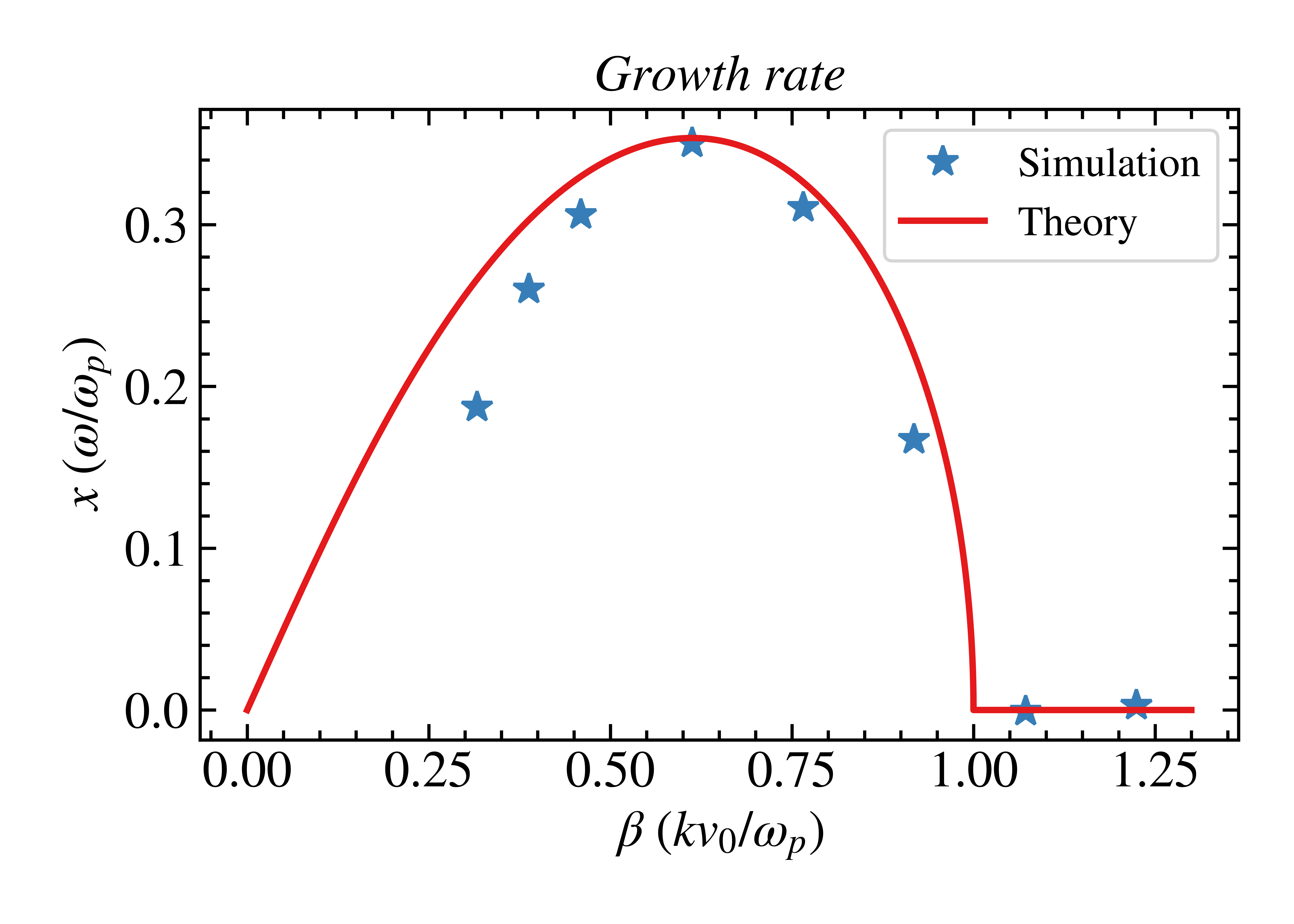
For two opposing moving electron beams with immobile ions as a background the dispersion relation gives: We can then verified that the growth rates of electric field in particular mode accord the theory we derive earlier.
\[\frac{\omega_p^2}{\left( \omega + \omega_D \right)^2} + \frac{\omega_p^2}{\left( \omega - \omega_D \right)^2} = 1\]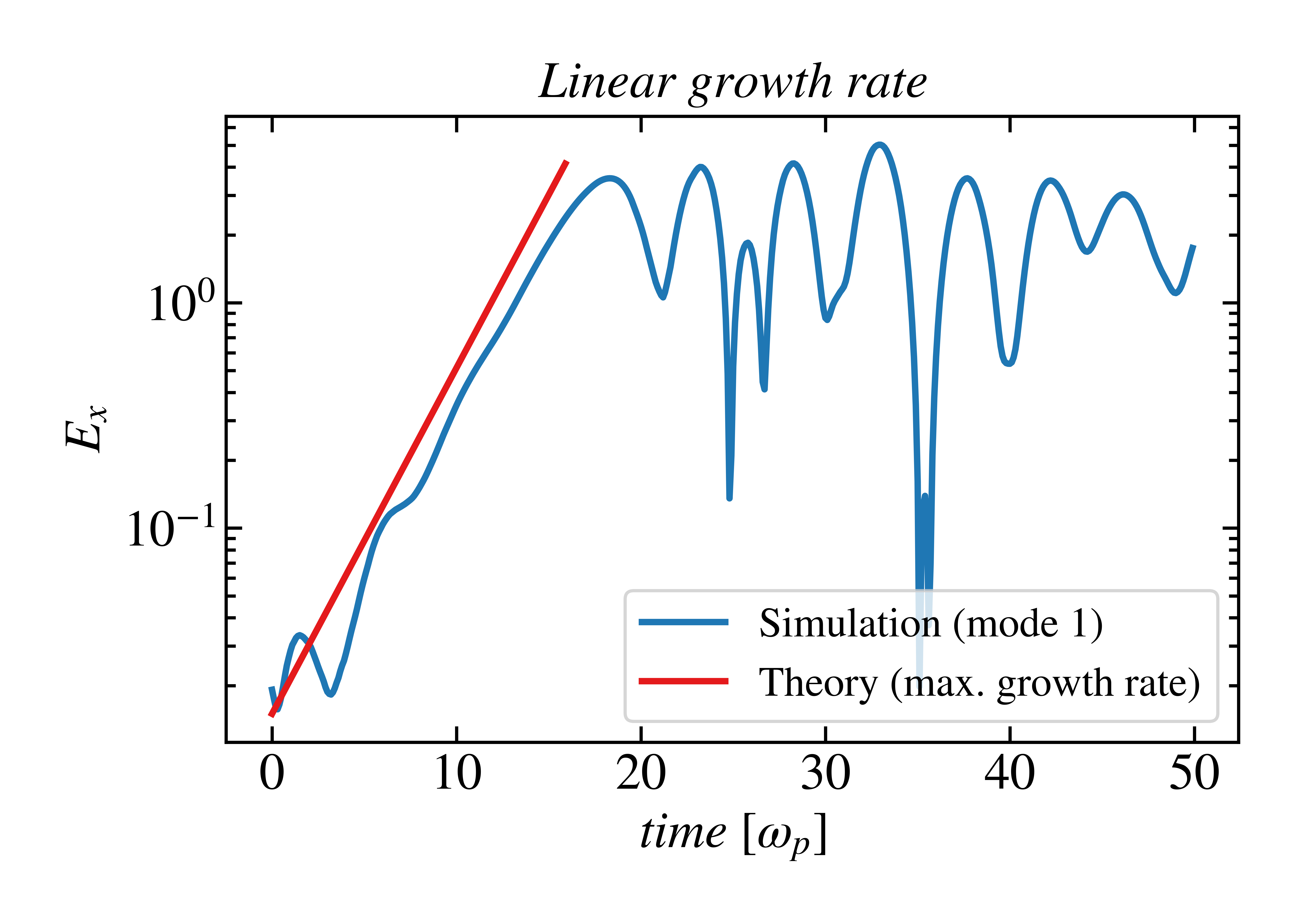
Finally we found out that in PIC simulation, mode with larger wave number are more consistence with theory, compare to small wave number mode which are more prone to competed with different modes in consequence of smaller growth rate than theory predict.